
In August 2022, CFD Direct introduced modular solvers to the development version of OpenFOAM (OpenFOAM-dev). Modular solvers are written as classes, in contrast to the traditional application solvers, integral to OpenFOAM since icoFoam in 1993. They are simpler to use and maintain than application solvers. Their source code is easier to navigate, promoting better understanding. They are more flexible; in particular, modules for different fluids and solids can be coupled across multiple regions, notably for conjugate heat transfer (CHT) with any type of flow, e.g. multiphase. Modular solvers are deployed using the foamRun or foamMultiRun applications, which contain a generic solution algorithm for single and multiple regions, respectively. Additional modules and applications replace existing tools for data processing and case configuration.
Application Solvers
OpenFOAM was originally conceived as a general development platform for computational fluid dynamics (CFD). Its creator, Henry Weller, exploited object orientation and generic programming in C++ to manage the complex science/engineering, mathematics and computing encountered in CFD. These programming paradigms minimise code duplication for more efficient maintenance. Data and functions are packaged in classes, with the functions providing a convenient interface to manipulate the data.
Most of the code in OpenFOAM is object-oriented and generic, i.e. contained within C++ classes and templates. It is divided across numerous libraries (~120 in OpenFOAM-v10), from the large core OpenFOAM and finiteVolume libraries to small libraries of physical models. By contrast, the application solvers contained a series of instructions that solved the governing equations within an iterative solution algorithm, and made function calls to various physical models, e.g. turbulence. The code was procedural, not object-oriented.
The Rise and Fall of Application Solvers
Over time, individual application solvers were customised for different categories of flow, e.g. incompressible, compressible, multiphase, etc. There were baseline solvers within each category, often with separate solvers for steady and transient flow. There were also variants of the baseline solvers which included combinations of: 1) additional modelling, e.g. porous media, dynamic meshes, Boussinesq’s approximation for buoyancy, single and multiple rotating frames (SRF and MRF), etc.; 2) numerics, e.g. local time stepping, different implementations of equation, the “consistent” option in pressure-velocity coupling, etc.
 Between the release of OpenFOAM v1.0 in 2004 and OpenFOAM v2.1 in 2011, the number of application solvers doubled from 41 to 82. While this established OpenFOAM across a broad range of CFD, the proliferation of solvers created its own problems. Users often struggled to choose between the different solvers. They then were forced to switch between solvers as they introduced new features into their simulations. They faced the daunting task of writing their own solver when none existed that included the particular combination of options they required. Code duplication was widespread, creating inconsistencies when a change to one application was not propagated through duplicate code in others.
To overcome these problems, CFD Direct generalised the optional modelling and numerics to move it out of the solver code. The number of solvers then decreased — along with the number of outstanding bugs — with users able to select the combination of options they wanted from their case configuration files. Some large components of OpenFOAM were significantly redesigned in the process, e.g. thermophysical transport, general models and constraints, and mesh motion, topology change and redistribution.
General Algorithm
When OpenFOAM v10 was released in 2022, the number of solvers has fallen to 48, close to the level in 2004. However, v10 solvers are very different to those from v1.0, since they contain modelling and numerics that did not exist in v1.0. They are much more complex, making them more difficult to maintain, and still including a lot of code duplication. It was natural, therefore, to turn to object orientation as the tried and tested approach of managing complexity and reducing code duplication.
The concept was to have one application, foamRun, to describe a general solution algorithm with functions that could be defined across a collection of modular solvers. Development of the idea was motivated by a need for a general method to couple solutions in multiple regions, containing different types of fluid and/or solid. The foamRun application for a single mesh region could be extended to a foamMultiRun application which executed the same functions across multiple mesh regions. Both applications contain the same algorithm with a time loop whose key functions are shown below (from foamRun.C)
while (pimple.run(runTime))
{
    solver.preSolve();
    adjustDeltaT(runTime, solver);
    runTime++;

    while (pimple.loop())
    {
        solver.moveMesh();
        solver.fvModels().correct();
        solver.prePredictor();
        solver.momentumPredictor();
        solver.thermophysicalPredictor();
        solver.pressureCorrector();
        solver.postCorrector();
    }

    solver.postSolve();
    runTime.write();
}
The functions in the algorithm are principally responsible for the following actions.
preSolve(): changes the mesh topology and maps between meshes.fvModels().correct(): updates the fvModels.moveMesh(): moves the mesh.prePredictor(): updates the fluid properties.momentumPredictor(): solves the momentum equation.thermophysicalPredictor(): solves an energy equation and updates thermodynamics.pressureCorrector(): solves a pressure equation.postCorrector(): solves the momentum transport, e.g. turbulence modelling, and thermophysical transport.postSolve(): cleans up, e.g. clearing temporary data.
Modular Solvers
The solver described in the code above forms the base class for a hierarchy of modular solvers shown below. Solver classes are derived from the base class, e.g. solid, fluidSolver. As the hierarchy is traversed from left to right, functions within the general algorithm (which begin as virtual functions in the solver class) are defined for different descriptions of fluids, e.g. incompressible, isothermal, multicomponent and multiphase. Sometimes the function is empty, e.g. thermophysicalPredictor() in the incompressibleFluid solver, since it does not include temperature. A lot of functionality is inherited by a derived class from its base class; in some case, base classes are created to define a general category of fluid, e.g. VoFSolver, whose functionality is inherited by four derived solvers based on the volume of fluid (VoF) method.
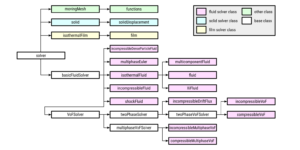
At the time of writing [updated: 2 May 2023], there are 13 fluid solvers, 2 film solvers, 2 solid solvers and 2 other solvers. These modular solvers replace the application solvers as follows.
- incompressibleFluid : supersedes pimpleFoam, pisoFoam and simpleFoam.
- isothermalFluid : supersedes potentialFreeSurfaceFoam using the waveSurfacePressure boundary condition.
- multicomponentFluid : supersedes reactingFoam and buoyantReactingFoam.
- fluid : supersedes rhoSimpleFoam, rhoPimpleFoam, buoyantFoam and coldEngineFoam.
- multiphaseEuler : supersedes multiphaseEulerFoam.
- compressibleVoF : is energy conserving and supersedes compressibleInterFoam and cavitatingFoam .
- incompressibleVoF :supersedes interFoam.
- incompressibleMultiphaseVoF : supersedes multiphaseInterFoam.
- compressibleMultiphaseVoF : supersedes compressibleMultiphaseInterFoam.
- shockFluid : supersedes rhoCentralFoam.
- XiFluid : supersedes XiFoam.
- incompressibleDriftFlux : supersedes driftFluxFoam.
- incompressibleDenseParticleFluid : supersedes denseParticleFoam.
- isothermalFilm : replaces surfaceFilmModels library.
- film : replaces surfaceFilmModels library.
- solid : replicates the solid region in chtMultiRegionFoam.
- solidDisplacement : supersedes solidDisplacementFoam and solidEquilibriumDisplacementFoam.
- movingMesh superseded moveMesh.
- functions : executes function objects in a time loop; with the scalarTransport function object it replicates scalarTransportFoam; and with the clouds fvModel, using incompressibleFluid and isothermalFluid as secondary solvers, it replicates particleFoam and rhoParticleFoam respectively.
- CHT is simulated by foamMultiRun with one or more fluid solvers and the solid solver, making chtMultiRegionFoam redundant; the compressibleInterPhaseThermophysicalTransportModel enables CHT with the compressibleVoF modular solver.
A modular solver can specified with foamRun through a solver keyword entry in the case controlDict file, e.g.
solver incompressibleFluid;
Alternatively, the solver can be specified using the -solver option when executing foamRun, i.e.
foamRun -solver incompressibleFluid
In addition to the modular solvers, two new applications have been created to replace functionality relating to application solvers.
- foamPostProcess utility : replicates the postProcess utility and the solver
-postProcessoption with modular solvers. - foamToC utility : replaces the
-list...options to locate models list their options.
Working with Modular Solvers
Through modular solvers, the benefits of object orientation are now extended to the solver component of OpenFOAM. Whereas application solvers presented equations, algorithm and model interface in a procedural manner, a modular solver is built around a generalised algorithm contained within the foamRun/foamMultiRun applications. Equations and interface are introduced at different levels of the class hierarchy. The solver for a particular fluid type includes little more than the code relating to that particular type. For example, the fluid solver is characterised by solving an energy equation in the thermophysicalPredictor() function, but otherwise inherits its functionality from the isothermalFluid solver.
It becomes clearer when using object orientation that a CFD solution involves time, space (mesh) and fields/properties that define the fluid/solid state. The foamRun/foamMultiRun applications initialise time and space and evolve time with the time loop. The moveMesh() function evolves space. Each modular solver represents a type of fluid/solid and is responsible for initialising and evolving the fluid/solid state within the pre-defined functions in foamRun/foamMultiRun. Developments focus on evolving the state properties specific to the particular fluid type, e.g. phase fraction in multiphase flow.
Modular solvers provide a distinct advantage for coupled solutions across multiple fluid and/or solid regions. Rather than writing customised application solvers for every combination of fluid and solid types, foamMultiRun allows any modular solver to be applied on any number of mesh regions. It is rapidly being adopted to calculate conjugate heat transfer with a variety of multiphase flows. Users no longer have an overwhelming choice of solvers, as their number decreases. Switching between steady and transient solutions no longer requires a change of solver. Physical models can be optionally selected through case configuration files, including buoyancy which is automatically activated by the presence of the p_rgh pressure field in the start-time directory.
Finally, the solvers in OpenFOAM capture the essence of its software design, 30 years after the first solver application, icoFoam, was written. As Andy Warhol once said: “